Environment map importance sampling
Environmental map is a common source of light in ray tracing applications. In bright day-time scenes, the ability to sample it efficiently is detrimental to reducing the noise. I want to share my experience with different ways of sampling. We assume that the environment is represented by a 2D image with pixels storing RGB floating point radiance. A value in a pixel represents the average radiance coming from any direction within the pixel area. The most redundant case for it being 1x1 white image. As for projection type, we are going to assume the Mercator projection.
The goal of a sampling routine is to generate a pseudo-random direction in 3D, together with the probability of how this direction was picked. That’s the basis of importance sampling. If our probability is correlated to the amount of energy that is coming from that direction, the lighting will converge fast.
struct Sample {
    dir: vec3<f32>, // sampling direction
    pdf: f32, // probability density in the unit of solid angle around the direction
}
All the experiments were conducted within blade engine. Shader code is in WGSL language.
Uniform

The simplest way to sample a direction is uniform: every direction is equally probable. However, there is a catch. If we just pick random azimuth (from -PI/2 to PI/2) and altitude, it’s not going to be uniform! Such a naive routine would oversample the poles of the sphere, because the amount of surface (on the sphere) changes as the cos(azimuth). The solution to this is to consider the height to be uniformly random. An interesting property of the sphere’s surface is that its area changes uniformly with the height: as we get closer to the poles, the radius decreases but the angle increases, which compensates it perfectly. I’ll leave the proof as an exercise to the reader - it’s fun, I highly recommend trying!
Let’s see how it can be expressed in the code:
let h = random();
let azimuth = 2.0 * PI * random();
// Distance from the center to the projection of the direction on XY plane
let r = sqrt(1.0 - h * h);
let dir = vec3<f32>(r * sin(azimuth), r * cos(azimuth), h);
// Density is such that the total integral across the sphere surface is 1
let pdf = 1.0 / (4.0 * PI);
return Sample(dir, pdf);
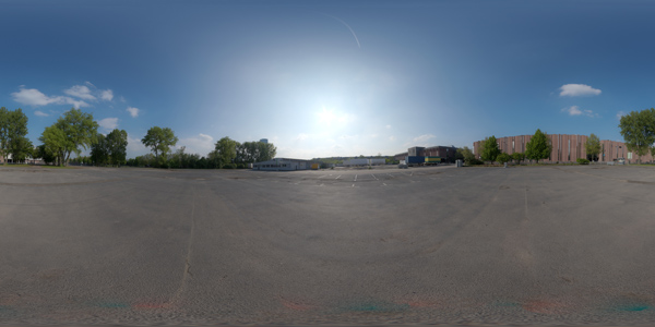
Uniform sampling is a great starting point, and also good for a backup plan when debugging more sophisticated algorithms. It’s easy to see where it fails: clear sky at day time would have most of the energy coming from the sun, and picking up that direction is not very likely with uniform sampling. That results in noise, lots of noise…
Important incident angle

At the end of the day, we are interested in maximizing the integral of the lighting equation, which is a product of the incoming light energy, its visibility, dot product with the surface normal, and the BRDF of the material.
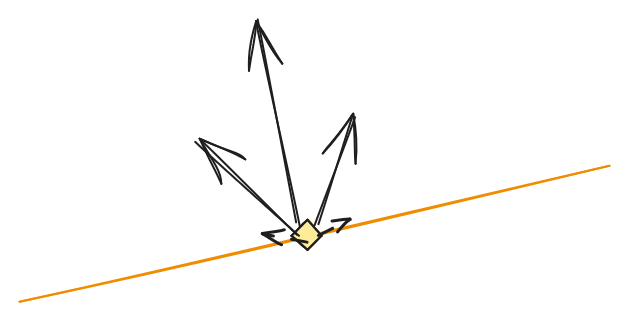
For importance sampling, we can consider some of these factors independently. The easiest one is the dot product of the light direction with the surface normal. We want the probability density to be proportional to the cosine of the angle between the light direction and the normal. Interestingly, this is the same cosine that broke the naive implementation of the uniform sampling! So all we need here is to choose the altitude naively, just sample in the space of the geometry surface.
let altitude = 0.5 * PI * random();
let azimuth = 2.0 * PI * random();
let local_dir = vec3<f32>(cos(altitude) * vec2<f32>(sin(azimuth), cos(azimuth)), sin(altitude));
// Normal is expected to match the local Z, so `sin(altitude)` = `cos(angle_with_normal)`
// Division by PI is to normalize the integral across the hemisphere to 1
let pdf = sin(altitude) / PI;
return Sample(local_to_world_rotation * local_dir, pdf);
This sampling works great when the other factors are more or less uniform. E.g. when the sky is covered in clouds, and there is similar amount of energy coming from any direction. It would converge faster than the uniform sampling in this case, but not in the case with a single bright sun in the sky.
Important light energy

Roughly speaking, if we are to choose between different factors to sample with importance, we should pick one that contains the least entropy. Or the most variation. The energy encoded into the environment light texture often has a lot of variation, and it comes with floating point 16 or even 32 bits of precision. Thus, it makes sense to pick the important texels to sample from when choosing the direction.
The task of importance sampling the texture belongs to the general class of discreet sampling algorithms. We have a set of texels, each with a corresponding energy value, and we want to importance sample them with probability that is proportional to the energy.
Hierarchical descent

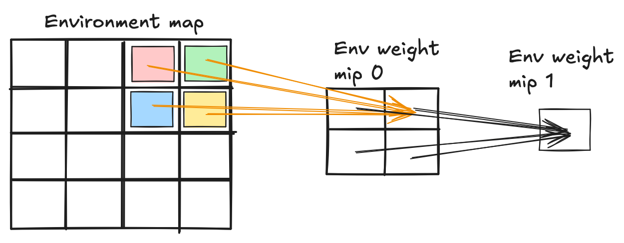
One way to do it is by starting with the highest mip level and then going through the mips down to the lowest level. Each step of the way we can randomly select one of the quadrants to follow. This method is used by the samples in RTXDI library from NVidia. I like it because it’s very intuitive, easy to imagine and reason about.
Preparation
In the preparation stage we need to build the mip chain. Each texel needs to contain 4 values: the total energy (or weight) of each of the quadrants in the 2x2 quad that this texel will be split into. The lowest mip is half the resolution of the original environmental map.
My preparation routine is just averaging the energy at each level, issuing a compute dispatch. For the original map, it computes the luminance value of the color. There is a catch, however. Since texels may cover different solid angles, computing the average energy requires us to weight them based on that solid angle:
let color = textureLoad(source, vec2<i32>(pixel), 0);
if (params.target_level == 0u) {
    let luma = max(0.0, dot(LUMA, color.xyz));
    let elevation = ((f32(pixel.y) + 0.5) / f32(src_size.y) - 0.5) * PI;
    let relative_solid_angle = cos(elevation);
    return clamp(luma * relative_solid_angle, 0.0, MAX_FP16);
} else {
    return dot(SUM, color);
}
I used “Rgba16Float” texture to store the values, but I can think of a better way. We could store 3 of the weights normalized in a texture like “Rgb10A2Unorm”. The last weight could be reconstructed automatically, and that would reduce the texel size from 64 bits to 32 bits.
Traversal
var pdf = 1.0;
var mip = i32(textureNumLevels(env_weights));
var itc = vec2<i32>(0); // texel coordinate
// descend through the mip chain to find a concrete texel
while (mip != 0) {
    mip -= 1;
    let weights = textureLoad(env_weights, itc, mip);
    let sum = dot(vec4<f32>(1.0), weights);
    let r = random_gen(rng) * sum;
    var weight: f32;
    itc *= 2;
    if (r >= weights.x+weights.y) {
        itc.y += 1;
        if (r >= weights.x+weights.y+weights.z) {
            weight = weights.w;
            itc.x += 1;
        } else {
            weight = weights.z;
        }
    } else {
        if (r >= weights.x) {
            weight = weights.y;
            itc.x += 1;
        } else {
            weight = weights.x;
        }
    }
    pdf *= weight / sum; // include the chosen probability
}

// adjust for the texel's solid angle
pdf /= compute_texel_solid_angle(itc, dim);
let dir = map_equirect_uv_to_dir(itc);
return Sample(dir, pdf);
The cost of this routine is proportional to log(largest_dimension). We are doing a texel fetch at each step.
Skip self-occlusion
This method can be improved by checking the texel areas against the surface normal. At each step of the descent, we can check if any of the texels are completely below the positive hemisphere, and reset their weight to 0. We could also lower the weight of texels base on how much they intersect with the lower hemisphere. This trick would make it much more likely to choose a direction that’s actually visible, at the cost of slightly more expensive descent.
Binary search
Another way to approach this is more general. Given a set of texels with their weight, we can compute the prefix sums for each. The weight of a texel is energy per solid angle. This precomutation can be done on CPU or GPU, it results in a large array of data:
struct EnvironmentTexel {
    weight_prefix_sum: f32,
    coordinates: vec2<i32>,
}
var<storage> env_texels: array<EnvironmentTexel>;
Then, for sampling, we just need to binary search a random value into this array, given that the prefix sums are strictly increasing. This gives us the inverse of a Cumulative Distribution Function (CDF) of the given probability weights.
let r = total_sum * random();
let index = binary_search(env_texels, r);
let et = env_texels[index];
let pdf = (env_texels[index + 1].weight_prefix_sum - et.weight_prefix_sum) / total_sum;
let dir = map_equirect_uv_to_dir(et.coordinates);
return Sample(dir, pdf);
The cost of this function is log(width * height), which is asymptotically the same as the previous method. There are numerous improvements that could be made here to increase the locality of access into the env_texels - something that the binary search is generally poor at.
Extra tricks
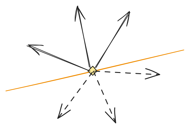
One unfortunate property of importance sampling based on light intensity is that it’s surface independent. I.e. it’s equally happy to pick a sample pointing “downwards” from the surface. That means, on average, half of the samples can be occluded immediately (and thus not useful).
Multiple samples
One easy trick to deal with that problem is to continue generating new samples for as long as they are occluded by the surface. This occlusion check is easy (we aren’t talking about a full shadow ray).
var num_samples = 0.0;
var estimate = vec3<f32>(0.0);
for (var i=0; i<5; i+=1) {
    let sm = generate_important_sample();
    num_samples += 1.0;
    // quickly check if it's self-occluded
    if (dot(sm.dir, normal) > 0.0) {
        let value = sample_environment(sm.dir);
        estimate = value / sm.pdf / num_samples;
        break;
    }
}
// now we can cast a real shadow ray
Equal area mapping

There are ways to map a square to a sphere’s surface with constant density. See practical implementation by Clarberg for details.
This mapping can be combined with another method (such as the binary search):
- pre-generate the 2D map (
energy_map) where each texel contains the total energy of the area that the equal area maps this texel into. - pre-generate an acceleration structure (such as the prefix sum array) for this 2D map.
- sample in 2 stages: first in precomputed energy map, then in the actual environment map.
Pseudo-code of the sampling algorithm:
struct MetaSample {
    vec2<i32> coords;
    float pdf;
}
// generate an important sample of the precomputed energy map
let equal_sample: MetaSample = pick_meta_sample(energy_map);
// Each texel maps to equal area of the sphere, divide by this area.
let pdf = equal_sample.pdf / constant_texel_area;
// Random offset within the texel.
let uv = (vec2<f32>(coords) + vec2<f32>(random(), random())) / vec2<f32>(textureSize(energy_map, 0));
let dir = equal_area_projection(uv);
return Sample(dir, pdf);
Learn the map
As it happens with problems that are difficult to solve algorithmically, we can resort to the mighty AI overlords. A neural network can learn the probability map of an environment map for a given surface orientation. Basically, the function:
probability(surface_normal, light_direction) = ?
I don’t understand the magic behind learning these probabilities yet, but it’s possible. It can be seen as learning the environment map itself at low resolution. I.e. the goal is to roughly understand which areas are bright, and what can be seen from a given perspective.
Random within
If the sampling produced a texel coordinate of the environment map (as opposed to purely a direction), it’s not the end. We need to generate a light direction, and it can come from anywhere covered by this texel. In the redundant case of 1x1 map, this can be the whole image! Thus, it may be required to randomly pick a direction within the texel area, to produce unbiased samples. I first tried to naively change the UV by random values within the texel:
let uv = (vec2<f32>(texel_coords) + vec2<f32>(random(), random())) / vec2<f32>(texture_size);
This works ok on large images but fails on small ones. This is due to the same problem of the density of the sphere surface being non-uniform, just now it’s within the texel as opposed to between texels. We need to take into account that latitude has the density of a cosine.
let u = (f32(texel_coords.x) + random_gen(rng)) / f32(texture_size.x);
let bounds = cos(vec2<f32>(vec2<i32>(texel_coords.y, texel_coords.y + 1)) / f32(texture_size.y) * PI);
let v = acos(mix(bounds.x, bounds.y, random_gen(rng))) / PI;
ls.uv = vec2<f32>(u, v);
Using this technique, my environment important sampling is unbiased for small images, even 1x1.
Afterword
Environment sampling is hard! Every method has trade-offs, and practical solutions are barely good enough. This is worsened by the fact that we often need to answer the question “how likely is this sample given our env sampling routine?” for the matter of Multiple Importance Sampling (MIS). Thus, it still shows up in profiles, and will probably remain the area of research for a while. In the meantime, hopefully, these pieces of code and descriptions help you to get things sampled :)
Edit: added “Equal area mapping” and “Skip self-occlusion” thanks to @ashpil’s feedback.